Visualizing geospatial BigQuery data with Elastic

Intro
I recently came across the Google Open Buildings dataset released in July 2021 and thought it would be nice to show we can visualize the buildings with Elastic. The dataset has been created by using computer vision on satellite imagery and includes ~516 million buildings and covers 64% of the whole African continent. All buildings are represented by polygons, with its footprint in square meters and a confidence score which tells us how certain the polygon is an actual building.
The Elastic Search Platform (Elastic Stack) is well suited to visualize this kind of geospatial data, and it’s quite easy too. There are several ways we could ingest the CSV data, for example with Filebeat or Logstash, but that would require us to install another component. If you’re already familiair with Google BigQuery it’s very easy to start ingesting and searching your data in Elasticsearch and Kibana. Elastic has native integrations with many GCP components, such as GCP Dataflow which can be used to send data in GCP to Elasticsearch.
GCP and BigQuery
First, we’re going to need an account on the Google Cloud Platform (GCP) and an Elastic cluster, which can be downloaded for free but the easiest way would be to create an Elastic Cloud cluster on GCP as well.
Next, we need to create a project (or use an existing one), I’ll name mine bigquery-elasticsearch and enable some APIs, namely BigQuery and Compute Engine.
Once we’re in BigQuery we can go ahead and create a new dataset, let’s call it openbuildings. On the Google Open Buildings website we can find all regions in Africa available in the dataset. For testing I would suggest to start with a smaller region, for example the one that covers northern Morocco and Algeria: https://storage.googleapis.com/open-buildings/data/v1/polygons_s2_level_4_gzip/0d7_buildings.csv.gz. To load this data to BigQuery we can run the following command in the GCP Cloud Shell Terminal:
bq load --autodetect openbuildings.data "gs://open-buildings-data/v1/polygons_s2_level_4_gzip/0d7_buildings.csv.gz"
The openbuildings part refers to the dataset that we want to use and the data part refers to the table we want the data to sit in. To check how it looks in tabular format we can preview it. It should look like this:

We can see that the polygon is in WKT format, which Elasticsearch can recognize automatically, so there is no need to transform the field values.
POLYGON((32.8112407240613 2.02121636012729, 32.8112435324021 2.02124311865723, 32.8112061858351 2.02124708622724, 32.8112033774958 2.02122032769721, 32.8112407240613 2.02121636012729))
Elasticsearch
If the BigQuery format looks good, we can continue with the Elasticsearch part. When dealing with geospatial data, and especially geoshapes, it is important to specify the index mapping so that it will not automatically map the geometry field to a text type. Using the Kibana Dev Tools we create the following request to make sure the geometry field is indexed as geo_shape type:
PUT openbuildings
{
  "mappings": {
    "properties": {
      "geometry": {
        "type": "geo_shape"
      }
    }
  }
}
Now when geospatial data is ingested with the field geometry it will be recognized as a geoshape. Even though the original dataset is in CSV, we can use the native GCP Dataflow integration to process and ingest the data into Elasticsearch as JSON documents. The geometry field consists of an array with all the polygon coordinate values and looks like this:
{
  "geometry": [
    "POLYGON((-5.60346473142983 36.012648155803, -5.60347842334872 36.012676425868, -5.60351392988928 36.0126650746182, -5.60350023795998 36.0126368045575, -5.60346473142983 36.012648155803))"
  ]
}
Ingestion
To start ingesting, we move over to the GCP Dataflow Console, create a new job from template, give it a name and a regional endpoint. The dataflow template we’re going to use is the BigQuery to Elasticsearch one.
Now we need to put in the Elasticsearch URL, an API key which can be created in Kibana Stack Management, and the targetted index name, e.g. openbuildings. In the optional parameters we will enter the table in BigQuery, which in my case is bigquery-elasticsearch:openbuildings.data. When that is all filled in, hit run job and it should start processing and ingesting the data into the Elasticsearch index. With a small dataset this could take a few minutes, but might depend on your setup and quotas.
Kibana Maps
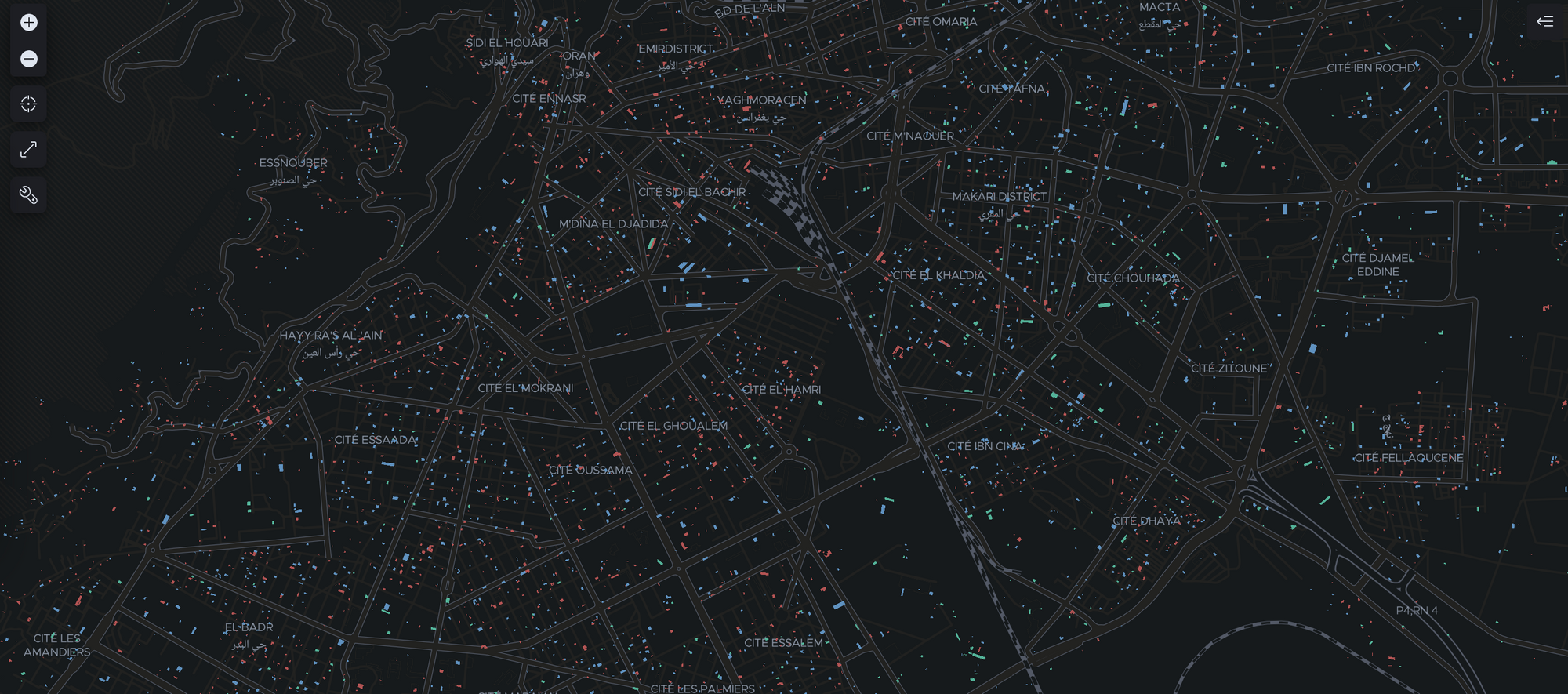
We can now check Kibana Stack Management again to see if all documents have been ingested and create the index pattern so Kibana can read and visualize the data in the index. To create the visualization as seen above, we go to Kibana Maps and add a new layer with documents from the index pattern. Depending on your preference, there is the possibility to limit to 10,000 results, show clusters, or use vector tiles (new feature). For now we’ll go with limit 10,000 results and zoom in on the city Oran in Algeria to have a look at the buildings there.
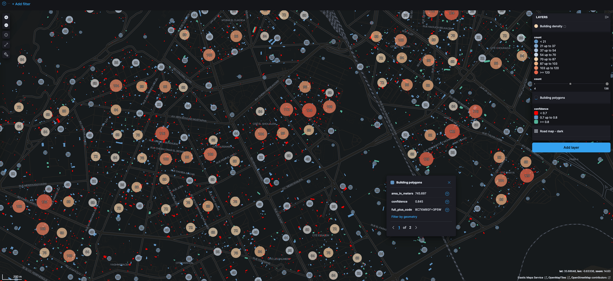
As a last step we can add different colors to the confidence scores and add another layer for clustering buildings based on their count (building density):

Now we can see an interesting map visualization which could be used as a base to enrich with more data and used for further analytics on for example population density, urban growth, or smart cities. All in all, this was a very smooth and easy process thanks to the native integrations between GCP and Elastic, Elasticsearch support for geoshapes, and easy geospatial visualizations in Kibana.